Applied Machine Learning
Four problem types, one discipline: baseline first, compare before choosing, then explain the choice.
- Context
- Machine Learning coursework, individual
- My part
- Everything: four notebooks and their write-ups
- Stack
- Python, scikit-learn, statsmodels, pandas
- Year
- 2025
The problem
Four assignments, four kinds of problem: predict when a factory machine is faulty, price a house, segment customers with no labels at all, and forecast three utilities five years ahead. Each one has an easy way to look good. Accuracy flatters a rare class, a random split leaks the future into a forecast, and a clustering score can be pushed up by adding features until the segments mean nothing.
So the work was less about finding the best model for each than about running the same discipline four times: set a baseline first, compare several models before choosing, keep the test data for one final look, and say plainly where the result is weak.
Forecasting gas, electricity and water
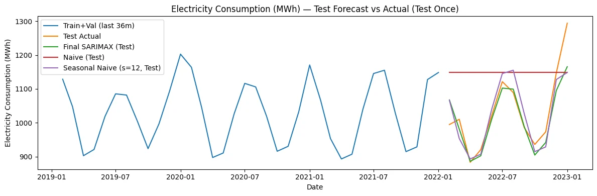
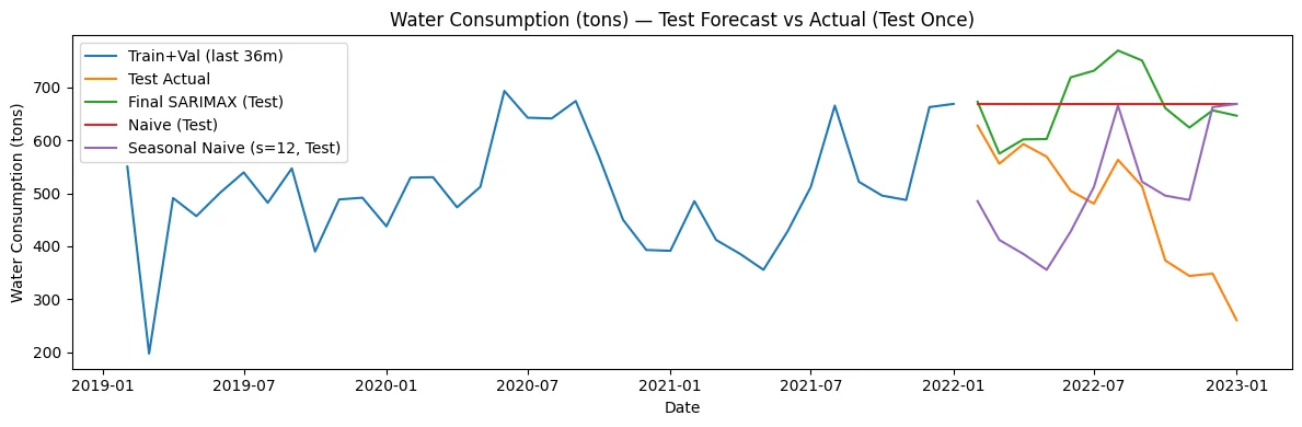
Monthly consumption from 1990 to 2023, 397 months with none missing, split in time order: 361 to train, the next 24 to compare and tune, the last 12 to test once. Every decision that could shape the model, from transforms to differencing, was made on training data only. Electricity’s spread grew with its level, so it was modelled on a log scale; gas and water stayed raw.
Naive and seasonal naive forecasts set the bar. ETS and SARIMAX were compared on validation, SARIMAX was tuned in two stages (a coarse grid, then a finer search around the best), and the winners were refit on train and validation before the single test.
Gas (tons)
Final model SARIMAX(3,1,3)(2,1,0,12)Test RMSE 2.91Best baseline RMSE 3.35, seasonal naive
Electricity (MWh)
Final model SARIMAX(2,0,0)(2,1,1,12)Test RMSE 48.47Best baseline RMSE 57.47, seasonal naive
Water (tons)
Final model SARIMAX(0,1,1)(2,1,0,12)Test RMSE 226.82Best baseline RMSE 193.40, seasonal naive
| Series | Final model | Test RMSE | Best baseline RMSE |
|---|---|---|---|
| Gas (tons) | SARIMAX(3,1,3)(2,1,0,12) | 2.91 | 3.35, seasonal naive |
| Electricity (MWh) | SARIMAX(2,0,0)(2,1,1,12) | 48.47 | 57.47, seasonal naive |
| Water (tons) | SARIMAX(0,1,1)(2,1,0,12) | 226.82 | 193.40, seasonal naive |
Gas and electricity beat both baselines. Water didn’t: a sharp drop late in the test year broke its pattern, and the model kept forecasting the old level. Its 60-month forecast drifts toward zero with a band that widens fast, and the notebook says to read it as a risk envelope, not a prediction.
Electricity, test year
Water, test year
Segmenting 200 customers
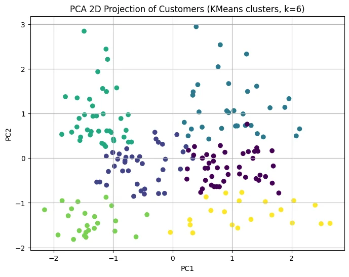
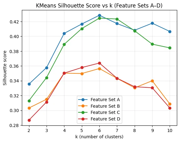
With no labels, one score can’t pick the answer. Three algorithms (KMeans, Gaussian mixtures and Ward clustering) were run on four feature sets, from age, income and spending alone to adding gender and an engineered spend-to-income ratio, for every k from 2 to 10. Candidates were judged on silhouette, the elbow in inertia, AIC and BIC for the mixtures, the smallest cluster’s share, and stability across repeated seeds measured with the adjusted Rand index.
KMeans, age/income/spend, k = 6
Silhouette 0.428Across seeds 0.428 ± 0.001, ARI 0.991Smallest cluster 10.5%
Ward, same features, k = 6
Silhouette 0.420Across seeds DeterministicSmallest cluster 10.5%
GMM, same features, k = 5
Silhouette 0.406Across seeds ARI 1.000Smallest cluster 11.5%
GMM, same features, k = 6 (rejected)
Silhouette 0.377Across seeds ARI 0.876Smallest cluster 6.5%
| Candidate | Silhouette | Across seeds | Smallest cluster |
|---|---|---|---|
| KMeans, age/income/spend, k = 6 | 0.428 | 0.428 ± 0.001, ARI 0.991 | 10.5% |
| Ward, same features, k = 6 | 0.420 | Deterministic | 10.5% |
| GMM, same features, k = 5 | 0.406 | ARI 1.000 | 11.5% |
| GMM, same features, k = 6 (rejected) | 0.377 | ARI 0.876 | 6.5% |
KMeans with six clusters on the three plain features won. Neither gender nor the engineered ratio earned its place, so both were left out. Profiling the six turned up the most useful segment: 33 customers with the highest income and some of the lowest spending, the clearest group to win over.
Silhouette by k
The six segments
Catching faulty machines
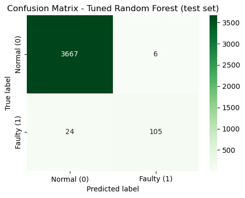
Twenty thousand readings of temperature, speed, torque and tool wear, where faults are 3.39% of rows after cleaning. A model that always says “normal” is 96.6% accurate and catches nothing, so every model was scored on F1 for the faulty class, with 5-fold stratified cross-validation on the training set and the test set kept for the end.
Random Forest
CV F1, baseline 0.843CV F1, tuned 0.881
Decision Tree
CV F1, baseline 0.827CV F1, tuned 0.827
SVM (RBF)
CV F1, baseline 0.436CV F1, tuned 0.795
| Model | CV F1, baseline | CV F1, tuned |
|---|---|---|
| Random Forest | 0.843 | 0.881 |
| Decision Tree | 0.827 | 0.827 |
| SVM (RBF) | 0.436 | 0.795 |
The tuned Random Forest reached F1 0.875 on the held-out test set: precision 0.946 and recall 0.814, so about four in five faults caught and few false alarms. Torque was its most important input.
Test confusion matrix
Pricing houses
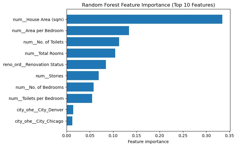
The smallest dataset, 545 houses, and the weakest result, reported as such. Prices were modelled on a log scale with three engineered features (area per bedroom, toilets per bedroom, total rooms) in one preprocessing pipeline. A tuned Random Forest edged a tuned Ridge on the test set: R² 0.502 against 0.498, MAPE 24.2% against 25.3%. Predictions still miss by about a quarter on average; house area and the engineered size features did most of the work.
What drove price
Decisions
Score the rare class, not the room
On the fault data, the do-nothing dummy is 96.6% accurate. Tuning on F1 for faults, and showing the dummy beside the final model, makes that number impossible to hide behind.
Split time in order, and test once
A random split would let the forecasts peek at the future. Train, validate and test run in sequence, the diagnostics only ever see training data, and the test year is used once, after the models are fixed, even when water came back worse than a baseline.
Earn every feature
Gender and the spend-to-income ratio were tested on every algorithm and k. When they didn’t improve quality or stability, they were dropped, so the final segments can be explained with the three numbers a marketer already has.
Stable beats a lucky peak
A clustering that changes with the seed can’t be acted on. The six-cluster mixture model scored reasonably once, but its assignments moved between seeds (ARI 0.876) and its smallest cluster was 6.5%, so it was rejected for the steadier KMeans.
Report the weak result as weak
Water losing to seasonal naive, residual autocorrelation left in two of three series, and a house-price model that explains half the variance all stay in the write-up. They show where these methods stop, which is the part a reader can trust.
Results
0.875
Test F1 on faulty machines, a class that is 3.39% of the data. The dummy scores 0
3.12%
Mean absolute percentage error forecasting electricity over a held-out year
0.991
Adjusted Rand index of the six customer segments across repeated seeds
Fault classification
Final model Tuned Random ForestHeld-out result F1 0.875, precision 0.946, recall 0.814
Forecasting, gas
Final model SARIMAXHeld-out result RMSE 2.91 vs 3.35 seasonal naive
Forecasting, electricity
Final model SARIMAX on log scaleHeld-out result RMSE 48.47 vs 57.47 seasonal naive
Forecasting, water
Final model SARIMAXHeld-out result RMSE 226.82, worse than seasonal naive at 193.40
Segmentation
Final model KMeans, k = 6Held-out result Silhouette 0.428, smallest cluster 10.5%
House prices
Final model Tuned Random ForestHeld-out result R² 0.502, MAPE 24.2%
| Problem | Final model | Held-out result |
|---|---|---|
| Fault classification | Tuned Random Forest | F1 0.875, precision 0.946, recall 0.814 |
| Forecasting, gas | SARIMAX | RMSE 2.91 vs 3.35 seasonal naive |
| Forecasting, electricity | SARIMAX on log scale | RMSE 48.47 vs 57.47 seasonal naive |
| Forecasting, water | SARIMAX | RMSE 226.82, worse than seasonal naive at 193.40 |
| Segmentation | KMeans, k = 6 | Silhouette 0.428, smallest cluster 10.5% |
| House prices | Tuned Random Forest | R² 0.502, MAPE 24.2% |
Coursework on the datasets we were given, not deployed models. Each result is one held-out split; there are no confidence intervals on the classification or regression scores.
Limits
- The forecasts use a single validation window, not walk-forward folds, so model choice rests on one two-year period.
- Electricity’s and water’s residuals still carry autocorrelation, and water’s long forecast goes negative, which no consumption can.
- The tuned Random Forest scores perfectly on its training data: it overfits, though its cross-validated and test F1 agree.
- Two hundred customers is a small base for six segments, and the personas are descriptions, not tested campaigns.
- The house-price model misses by about 24% on average; it explains the drivers better than it predicts a price.